Basics of iactsim

Build an optical system

In iactsim, an optical system is a collection of optical surfaces. To build one, you first define the individual components of your telescope and then group them together using the OpticalSystem class.

Because the ray-tracing kernel uses a non-sequential ray-tracing approach, you do not need to worry about the exact order in which you provide the surfaces. As a photon travels, the simulation automatically determines its path by checking the nearest surface whose bounding sphere the ray will intersect next.

In this tutorial we are going to define a simple telescope consisting of a spherical primary mirror and a flat sensitive camera at the focal plane.

Defining surfaces

Every component in your system is represented by a Surface object. iactsim provides different built-in shapes (like FlatSurface, SphericalSurface, or AsphericalSurface) and types (such as REFLECTIVE, REFRACTIVE, or SENSITIVE).

Apart from the specific initialization values required by their geometry (such as radius, height, or aspheric coefficients), all surfaces share these core properties:

• surface_type (SurfaceType): defines the functional behavior of the surface (e.g., REFLECTIVE, SENSITIVE, OPAQUE).

• position (array-like): the [x, y, z] coordinates of the surface center in the telescope reference frame.

• tilt_angles (array-like): the [x, y, z] counter-clockwise rotation angles in degrees.

• material_in and material_out (Material): define the optical media bounding the surface. Their exact meaning depends on the class type (i.e., whether it is an open surface or a closed shape like a BoxSurface or CylindricalSurface).

• properties (SurfaceProperties): object defining reflectance, transmittance and absorption profiles.

• scattering_dispersion (float): standard deviation for simulating Gaussian deviation for the surface normal.

• visual_properties (SurfaceVisualProperties): attributes to customize how the surface looks in the 3D visualizer.

• name (str): a custom string identifier for the surface.

Define a mirror

First, we instantiate the primary mirror of our telescope using the SphericalSurface class. By setting its surface_type to REFLECTIVE, we tell the engine that photons hitting this surface should be reflected.

We place the mirror at the origin of the telescope reference system ([0.0, 0.0, 0.0]). For its geometry, we define a 10-meter diameter and a 20-meter radius of curvature (i.e. a focal length of 10 meters).

from iactsim.optics import (
    SphericalSurface,
    SurfaceType
)

# Spherical mirror properties
mirror_curvature_radius = 20_000. # mm
plate_scale = mirror_curvature_radius/57.296/2. # mm/deg
half_aperture = 10_000. # mm

# Initialize the surface object
mirror = SphericalSurface(
    half_aperture=half_aperture,
    curvature=1./mirror_curvature_radius,
    position=(0,0,0),
    surface_type=SurfaceType.REFLECTIVE,
    name='Mirror'
)

Define a sensitive surface

Next, we define the focal plane of our telescope using a FlatSurface. By assigning it the SurfaceType.SENSITIVE type, we designate this surface as a detector that will record the photons that hit it.

Warning: An OpticalSystem requires at least one sensitive surface to be initialized. Without a detector, the ray-tracing engine has no endpoint to collect the simulation results and will raise an error. In this example, we place a flat focal-plane surface exactly at the mirror focal length.

from iactsim.optics import (
    FlatSurface,
    ApertureShape
)

focal_plane_inradius = 3. * plate_scale # mm
focal_plane = FlatSurface(
    half_aperture=focal_plane_inradius,
    aperture_shape=ApertureShape.HEXAGONAL_PT,
    surface_type=SurfaceType.SENSITIVE,
    position=(0,0,0.5*mirror_curvature_radius),
    name='FocalPlane'
)

Instantiate the optical system

Now that our individual components are defined, the final step is to assemble them using the OpticalSystem class.

To do this, you simply pass a list of surface objects to the constructor.

In a Jupyter Notebook, evaluating the os object will automatically render a formatted HTML table summarizing your optical system.

from iactsim.optics import OpticalSystem

os = OpticalSystem(
    [mirror, focal_plane],
    name='MyOS'
)

os

Optical System: MyOS

Surface Name	Axial Position	Material 1	Material 2	Surface Type
Mirror	0	AIR	AIR	REFLECTIVE
FocalPlane	10000	AIR	AIR	SENSITIVE

Understanding curvature and “front/back” convention

When building your optical system, it is important to understand how iactsim handles the orientation of curved surfaces and direction-specific interactions within the surface local reference frame:

• Curvature: the sign of the curvature parameter defines the geometric shape of spherical and aspherical surfaces. If the curvature is positive, the mirror is concave towards the positive z-direction (in the surface reference frame).

• Front/back: by default, base surface types like SurfaceType.REFLECTIVE or SurfaceType.SENSITIVE interact with photons hitting them from both sides. To restrict interaction to one side, use the _FRONT or _BACK variants:

  • _FRONT types: only interact with photons arriving with a negative z-component in the surface reference frame. For closed surfaces (such as BoxSurface or CylindricalSurface), this corresponds to light arriving from the outside.

  • _BACK types: only interact with photons arriving with a positive z-component in the surface reference frame. For closed surfaces, this corresponds to light arriving from the inside.

  The other side becomes “OPAQUE” (i.e. photons that reach the surface are killed).

Advanced surface optical properties definition

With iactsim you can achieve a more generic treatment of any surface by setting its type to SurfaceType.REFRACTIVE and/or SurfaceType.REFLECTIVE_SENSITIVE and defining specific surface properties to handle refraction, transmission, absorbtion and detection explicitly for both surface sides.

However they are out of the scope of this introductory tutorial.

Visualize the geometry

Note: The interactive 3D visualizer relies on the vtk library, which is an optional dependency and is not installed by default with iactsim. Before running this step, ensure you have installed it in your environment: pip install vtk

When building a 3D setup it is highly recommended to visually verify your geometry to ensure every component is oriented exactly as you intend.

Using the built-in VTK visualizer, you can easily render an interactive 3D view of your optical system to inspect its alignment (for example, by visualizing a surface reference system orientation):

from iactsim.visualization import VTKOpticalSystem

vtk_os = VTKOpticalSystem(os)
vtk_os.start_render()

Mirror segmentation

While you could calculate the 3D position and rotation matrix for each segment, the offset attribute provides a direct mechanism to handle this. Using offset it is possible to model segments when the primary mirror has a non-spherical shape (such as an aspherical surface, since an off-axis cutout does not share the same symmetrical geometry as the center of the mirror).

When you assign an [x, y] offset to a surface, the engine treats it as a segment located at those coordinates on the parent mirror and it automatically computes the correct local surface normal for that specific spot. The segment is an independent surface that can be positioned everywhere and, because the ideal alignment is handled natively by the offset, the tilt_angles parameter acts as a misalignment error relative to its ideal orientation.

In the example below, we generate a grid of square mirror segments, apply a random tilt misalignment and surface scattering (i.e. a deviation from the nominal surface normal) to each, and finally remove our original monolithic mirror from the system:

import numpy as np

# Segment ID
k = 0

# Segments on a 10X10 grid
n = 10
segment_distance = 2*mirror.half_aperture / (n+3)

for i in range(n+3):
    for j in range(n+3):
        offset = [
            -mirror.half_aperture+segment_distance*i,
            -mirror.half_aperture+segment_distance*j
        ]
        r_segment = np.sqrt(offset[0]**2+offset[1]**2)

        # Do not create segments outside the original mirror aperture
        if r_segment > mirror.half_aperture-segment_distance*np.sqrt(2):
            continue

        # Ideal segment position
        segment_position = [
            offset[0],
            offset[1],
            mirror.sagitta(r_segment),
        ]

        # Create the surface
        segment = SphericalSurface(
            curvature=mirror.curvature,
            half_aperture=0.45*segment_distance,
            position=segment_position,
            surface_type=mirror.type,
            name = f'MirrorPanel{k}',
            aperture_shape=ApertureShape.SQUARE,
            # Big random dispersion for visualization purpose
            tilt_angles=np.random.uniform(0,0.05,3),
            # Gaussian dispersion of the normal vector of the surface, in degrees
            scattering_dispersion=0.02
        )

        # Specify the segment offset
        # When a segment is created in this way:
        #  - it will be oriented with the same surface normal
        #    of the mother surface at the specified offset
        #  - `tilt_angles` attribute will define a deviation from this orientation.
        segment.offset = offset

        os.add_surface(segment, replace=True)
        k += 1

os.remove_surface('Mirror')

Re-initialize the visualizer

vtk_os = VTKOpticalSystem(os)
vtk_os.start_render()

Set up the telescope for ray-tracing

With the optical system fully assembled, the final setup step is to link it to the simulation engine using the IACT class.

The IACT object acts as the master controller for your simulation. It wraps your optical system, sets the global 3D position of the telescope and manages its pointing direction (defined by altitude and azimuth in degrees). It also manages GPU-CPU data transfers required to perform the actual ray-tracing, which is executed via CUDA kernels under the hood.

Because of this GPU-accelerated architecture, you must call the cuda_init() method after defining your telescope (and after any change of a surface property). This function compiles your entire optical configuration, computes the necessary transformation matrices, and transfers all the geometric and material data directly into the GPU memory so it is ready for ray-tracing.

from iactsim import IACT

telescope = IACT(
    os,
    position=(0.,0.,0.),
    pointing=(0.,0.)
)

telescope.cuda_init()

Reference systems

To accurately simulate light propagation, iactsim relies on a strict hierarchy of 3D coordinate systems. As a photon travels through the simulation, its coordinates are sequentially transformed through three distinct frames: local → telescope → surface.

The local reference system

This is the global, ground-based environment (similar to the CORSIKA reference system). It is defined as a fixed North-West-Up coordinate system:

• X-axis: points North (Azimuth = 0°)

• Y-axis: points West (Azimuth = 270°)

• Z-axis: points to the Zenith (Altitude = 90°)

The telescope reference system

This frame moves with the telescope as it points in the sky. The transformation from the local frame to the telescope frame is defined by the telescope current Altitude and Azimuth.

By default, when the telescope points at the horizon towards the North (Alt=0, Az=0), the axes are aligned as follows:

• Z-axis: aligned with the telescope optical axis, pointing North.

• X-axis: perpendicular to the optical axis, pointing downward.

• Y-axis: perpendicular to the optical axis, pointing West.

Note: If this default orientation does not match your specific instrument geometry, you can assign a rotation matrix to the custom_rotation attribute of the IACT object.

Ray-tracing example: visualize spot diagrams

To evaluate the optical performance of our telescope, we can simulate a uniform beam of light and visualize the resulting spot diagram at the focal plane. We do this using the Source class.

On-axis photon source

The Source class acts as a customizable photon generator. When you initialize it by passing your telescope object, it automatically sets itself up as a uniform disk of light positioned high above the system.

Under the hood, a Source manages four distinct generators for the photons:

• positions: where the photons originate (defaults to a uniform disk).

• directions: which direction they travel (defaults to a parallel beam matching the telescope pointing).

• spectrum: their wavelengths (defaults to a uniform distribution).

• arrival_times: when they start their path, i.e. the arrival time at the source surface (defaults to a constant time).

In the code below, we create the source and use set_target([0, 0, 0]) to precisely aim the center of the beam at the origin of our optical system, creating an ideal on-axis light source:

from iactsim.optics import sources

source = sources.Source(telescope)
source.set_target([0,0,0])

Run the ray-tracing

First, we call source.generate() to create a batch of photons. This method returns four arrays representing the initial state of our light beam:

• ps: 3D positions

• vs: 3D direction vectors

• wls: wavelengths

• ts: times

Next, we feed these arrays directly into the telescope.trace_photons() method. This triggers the CUDA-accelerated ray-tracing kernel:

# Generate photons
ps, vs, wls, ts = source.generate(100_000)

# Perform ray-tracing
telescope.trace_photons(ps, vs, wls, ts)

Internal GPU Arrays

When you pass standard NumPy arrays to trace_photons(), the method automatically allocates dedicated CuPy arrays on the GPU to store the results.

After the simulation runs, you can access the final state of the photons using the following internal attributes of the IACT object:

• _d_positions: an (N, 3) array containing the final coordinates of each photon.

• _d_directions: an (N, 3) array containing the final direction vectors.

• _d_wavelengths: an (N,) array of the photon wavelengths (in nm).

• _d_arrival_times: an (N,) array of the final arrival times (in ns).

If a photon doeas not reach a sensitive surface during ray-tracing its state variables are set set to NaN.

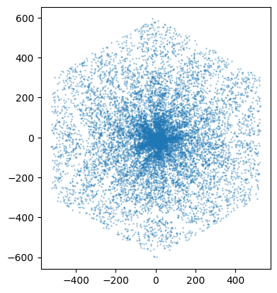
Visualize detected photon position

Since Source.generate() returns cupy arrays, trace_photons() passes them directly to the CUDA kernels for in-place modification. In this case the ps and _d_positions arrays point to the same GPU memory buffer:

from iactsim.visualization import scatter

scatter(ps)

Visualize ray-tracing

To visualize the ray-tracing through the optical system, you can use the visualize_ray_tracing() method (based on the built-in VTK visualizer). This allows you to see the full 3D trajectory of photons as they propagate through the optical system:

telescope.visualize_ray_tracing(
    *source.generate(100_000),
    map_wavelength_color=False,
    focal_point='FocalPlane'
)

Defining a custom pixel module with the GenericFlatModule class

Key concepts

• Pixel-level control: each pixel in a GenericFlatModule is an independent GenericPixel object. This allows you to mix different pixel shapes, sizes and optical properties (reflectance and efficiency) within the same module.

• Module geometry: the module itself has an outer boundary (defined by half_aperture and aperture_shape) and can include a central hole. The class includes a check_pixels_contained() method to ensure your pixel layout physically fits within these boundaries.

• GPU integration: When you call telescope.cuda_init(), the module automatically packs the geometry and optical tables of all its pixels into structured arrays and uploads them to GPU memory.

In order to define a module you must create a list of GenericPixel objects. Each pixel must be initialized with its relative \((x, y)\) coordinates in the surface reference frame, its shape, its half-aperture size and a unique identifier.

For example in the following we are going to fill an hexagonal module with hexagonal pixels:

def is_inside_hexagon(x, y, inradius, pointy_top=True):
    px, py = abs(x), abs(y)

    if pointy_top:
        px, py = py, px

    if py > inradius:
        return False

    return (px * np.sqrt(3) + py) <= (2.0 * inradius)

from iactsim.optics import GenericPixel

pixels = []
half_size = 10.0  # Inradius of the pixel (mm)
separation = 1.  # Gap between pixels (mm)
camera_inradius = focal_plane_inradius
pixel_id = 0

eff_half_size = half_size + (separation / 2.)
circumradius = (2 * half_size) / np.sqrt(3)

allowed_inradius = camera_inradius
camera_circumradius = (2 * camera_inradius) / np.sqrt(3)
max_steps = int(camera_circumradius / eff_half_size) + 2

for j in range(-max_steps, max_steps + 1):      # Rows (y-axis)
    for i in range(-max_steps, max_steps + 1):  # Columns (x-axis)

        # Stagger every other row
        x_offset = (j % 2) * eff_half_size
        x_pos = i * (2 * eff_half_size) + x_offset
        y_pos = j * (np.sqrt(3) * eff_half_size)

        # Check if the pixel center is within the camera boundary
        if is_inside_hexagon(x_pos, y_pos, allowed_inradius, pointy_top=True):
            pixel = GenericPixel(
                x=x_pos,
                y=y_pos,
                half_size=half_size,
                shape=ApertureShape.HEXAGONAL_PT,
                pixel_id=pixel_id,
            )
            pixels.append(pixel)
            pixel_id += 1

How to define a GenericFlatModule object

The module must be initialized with a list of GenericPixel objects fully contained on the surface:

from iactsim.optics import GenericFlatModule

module0 = GenericFlatModule(
    pixels=pixels,
    half_aperture=camera_inradius+5*separation,
    aperture_shape=ApertureShape.HEXAGONAL_PT,
    surface_type=SurfaceType.SENSITIVE_BACK,
    position=focal_plane.position,
    tilt_angles=(0,0,0),
    name='Module0'
)

Integrate it in the optical system

os.add_surface(module0, replace=True)
os.remove_surface('FocalPlane')

telescope.cuda_init()

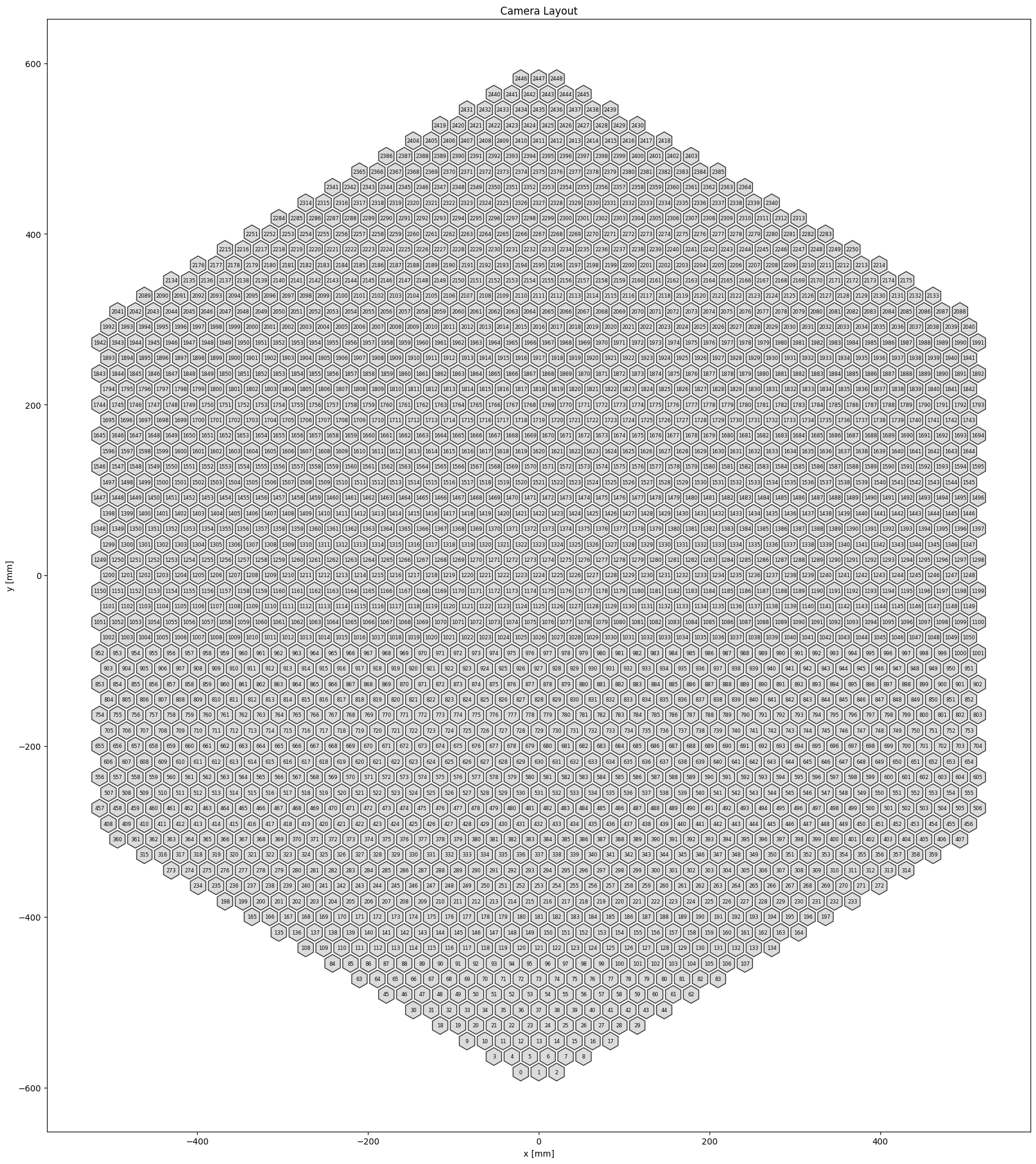
Check the camera layout

After defining your module (or modules), you should verify that the pixels are correctly positioned in the telescope coordinate system. The CameraGeometry class extracts this information from the telescope object, automatically handling 3D rotations and offsets for every sensor.

Use plot_layout() method to generate a 2D visualization:

from iactsim.optics import CameraGeometry

cam_geo = CameraGeometry(telescope)
_ = cam_geo.plot_layout()

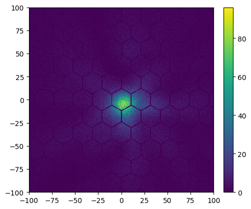
Visualize detected photons

You can also check the simulation results using the histogram2d function:

from iactsim.visualization import histogram2d

telescope.trace_photons(*source.generate(10_000_000))
hist, ax = histogram2d(telescope._d_positions, 400, log=False, range=[[-100,100],[-100,100]])

Multiple modules and pixel ID requirements

iactsim supports any number of module instances (both GenericFlatModule and SipmTileSurface) within a single optical system. This allows for the construction of modular cameras.

To ensure the ray-tracing kernels, electronics kernels, and visualization functions work correctly, pixel identification must follow two rules:

• uniqueness: every pixel in the optical system must have a unique pixel_id. The CameraGeometry class will raise a ValueError if it detects a duplicate ID across different modules;

• range: pixel IDs must be contiguous and assigned within the range \([0, N-1]\), where \(N\) is the total number of pixels in the system.

Note: When using SipmTileSurface, pixel IDs are assigned sequentially starting from the value of the attribute first_pixel_id. This atribute should be correctly set to prevent ID collisions.

Camera simulation

Get input for the camera simulation

Now that we have traced our photons through the telescope optical system, the next step is to simulate how the camera electronics respond to this light.

Before we run the full camera simulation, it is helpful to understand the raw data that feeds into it. The trace_photons() method includes a get_camera_input argument. When enabled, the method returns the arrays needed to simulate the electronics response: the photon arrival times and a pixel mapping array:

pes, mapping = telescope.trace_photons(
    *source.generate(10_000_000),
    get_camera_input=True
)

Note: trace_photons() can handle also multi-event simulations by computing a specific mapping for each event, but it is not treated in this tutorial.

Where:

• pes: a flat 1D array containing the arrival time of every single photon that has been successfully detected by a camera pixel;

• mapping: ndarray with shape (n_events, n_pixels+1,) of first and last arrival time position inside pes for each pixel in each event (e.g. arrival times on pixel k → pes[mapping[k]:mapping[k+1]]).

Because mapping is a cumulative sum, we can calculate the number of photons that arrived at each individual pixel by taking the discrete difference for a given event. Here we get the first element of the mapping, which corresponds to the first event (the only one in this case):

n_pes = np.diff(mapping[0])

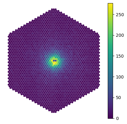
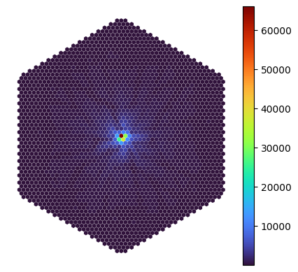
Visualize camera images

Now that we have a 1D array containing the total number of photoelectrons in each pixel, we can visualize these values on the focal plane.

We can use the camerashow function, which takes our 1D array of pixel values and maps it onto the camera layout using the CameraGeometry object we defined earlier:

from iactsim.visualization import camerashow

_ = camerashow(n_pes, cam_geo, cmap='turbo')

Define a SiPM camera

Before we can process the photon arrival times we generated in the previous step, we need to define how the camera electronics respond to those photons. In a real Silicon Photo-Multiplier (SiPM) camera, a single arriving photon triggers an avalanche that is shaped by the electronics into a specific electrical pulse.

In our simulation, each detected photon is assumed to result in a signal of the exact same shape. When multiple photons arrive at a pixel within a given time window, their individual pulses simply superimpose to construct the global waveform for that channel.

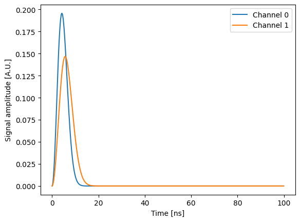
So, we need to define this “single-photoelectron waveform” for our channels using the Waveform class. Here, we will define a generic, dummy pulse shape and create a two-channel camera:

• Channel 0: a slightly faster pulse, which we will use for our trigger logic;

• Channel 1: a slightly wider pulse, which we will use for our signal sampling.

from iactsim.electronics import Waveform

def dummy_pulse(extent, resolution, peak_delay, sigma):
    t = np.arange(0, extent, resolution)
    z = (t - peak_delay) / sigma
    log_norm = -0.5 * (z**2 + np.log(2*np.pi)) - np.log(sigma)
    y = np.where(log_norm<10, t**2*np.exp(log_norm), 0)

    wave = Waveform(t, y, 'DC')
    wave.normalize()
    return wave

waveforms = (
    dummy_pulse(100, 0.1, 0, 3),
    dummy_pulse(100, 0.1, 0, 4),
)

import matplotlib.pyplot as plt

plt.xlabel('Time [ns]')
plt.ylabel('Signal amplitude [A.U.]')
plt.plot(waveforms[0].time, waveforms[0].amplitude, label='Channel 0')
plt.plot(waveforms[1].time, waveforms[1].amplitude, label='Channel 1')
_ = plt.legend()

Define trigger and sampling logic

The following implements a camera where

• channel0 is a trigger channel

• channel1 is a sampling channel

• the trigger follows a ‘majority’ logic (n pixels above a given signal)

• the sampling performs a sum of the pixel signal in a 32 ns window starting 10 ns before the camera trigger

The trigger window extent is computed from the photon arrival times. To take into account the electronics shape of the signal, the window must be extented accordingly using the attribute trigger_window_end_offset.

Defining Trigger and Sampling Logic

The iactsim framework uses abstract classes like CherenkovSiPMCamera to handle low level core tasks (like time-window management, background noise and cross-talk computation on the GPU). To create our specific camera, we just need to inherit from this class and implement two key methods: trigger_action() and sampling_action().

Here is the logic we want to implement for our DummySiPMCamera:

• Trigger: the camera will use a majority trigger logic. It will look at all pixels simultaneously in each time bin. If more than majority_nn pixels cross a signal threshold of threshold, the camera considers it a valid event and triggers. The trigger_action() method, upon a camera trigger, must set the trigger_time and triggered attribute.

• Sampling: Once triggered, the camera needs to digitize the signal. It will look at Channel 1 and integrate the signal over a 32 ns window. To make sure we capture the whole pulse, this window will start 10 ns before the trigger time. The integral is computed directly from the channel signal, no actual digitization is performed in this example.

from iactsim.electronics import CherenkovSiPMCamera
import cupy as cp

class DummySiPMCamera(CherenkovSiPMCamera):
    def __init__(self, n_pixels, waveforms, channels_time_resolution):
        super().__init__(
            n_pixels = n_pixels,
            waveforms = waveforms,
            channels_time_resolution = channels_time_resolution,
            trigger_channels = [0],
            sampling_channels = [1]
        )

        # CherenkovSiPMCamera attributes
        self.sampling_window_extent = [32.] # ns (one for each sampling channel)
        self.sampling_delay = [-10.]
        self.trigger_window_end_offset = [30.]
        self.trigger_window_start_offset = [0.]

        # New attributes
        self.images = []
        self.majority_nn = 4
        self.threshold = 5
        # The threshold unit must be consistent with the gain (1 in this dummy case)

    def restart(self):
        super().restart()
        self.images.clear()

    def trigger_action(self):
        # Shape (n_pixels, window_size)
        signal = self.get_channel_signals(0, reshape=True)

        # Check if there is a time bin where at least `majority_nn` pixels are over a given value
        counts = cp.count_nonzero(signal>self.threshold, axis=0) # Shape (window_size,)
        trigger_time_slice = cp.argmax(counts>self.majority_nn).get() # Move to the host in order to use it as an index

        # argmax returns 0 if all values are 0
        if trigger_time_slice == 0:
            if not cp.any(counts>self.majority_nn):
                return

        # Get the trigger time (from the channel 0 time window)
        self.trigger_time = self.time_windows[0][trigger_time_slice]
        self.triggered = True

    def sampling_action(self):
        # Shape (n_pixels, window_size)
        signal = self.get_channel_signals(1, reshape=True)
        # Shape (n_pixels,)
        image = cp.sum(signal, axis=1)
        # Save the image
        self.images.append(image)

Inheriting from CherenkovSiPMCamera

When you write a custom camera class, you inherit from CherenkovSiPMCamera. To ensure the underlying logic works properly, you need to handle two setup steps:

• the constructor (__init__()): the base classes manage GPU memory allocation and internal state variables. You must call super().__init__() to pass your core configuration (pixels, waveforms and channels) to the base class. Once the base framework is initialized, you can define your custom camera parameters, such as self.images, self.threshold and your time window offsets.

8 the restart() method: when running sequential simulations, you can call restart() to clear old data like event counters and previous trigger times. To override this method the super().restart()call is needed, after this call you can clear any custom data your camera accumulated during the run. In our case, this means emptying the self.images list.

Accessing the signals

In both the trigger and sampling logic, we access the waveform data using get_channel_signals() method.

iactsim stores the simulated waveforms for all pixels and channels in a single 1D array (signals). The get_channel_signals() method handles the memory mapping to retrieve the specific data for the requested channel. Using the reshape=True argument returns this data as a 2D CuPy array with shape (n_pixels, window_size).

Because the returned signal is a 2D CuPy array on the GPU, you can evaluate the entire focal plane simultaneously using vectorized operations instead of Python for loops. For example:

• cp.count_nonzero(signal > self.threshold, axis=0) counts how many pixels cross the threshold in each time bin;

• cp.sum(signal, axis=1) integrates the waveform across the time window for every pixel, resulting in the final 1D image array.

Note: Unlike the trigger channel signals, which are always computed, the sampling channel signals are computed only if a trigger occurs. So you should not access the signal of these channels inside trigger_action().

Assign the camera to the telescope

Now we just need to instantiate a DummySiPMCamera object and assign it to the camera attribute of our IACT object:

camera = DummySiPMCamera(
    n_pixels = cam_geo.n_pixels,
    waveforms = waveforms,
    channels_time_resolution=[1,1] # 1 ns resolution for both channels
)

telescope.camera = camera

SiPM properties

The CherenkovSiPMCamera class allows you to define pixel-specific parameters to simulate the physical behavior and noise characteristics of real Silicon Photo-Multipliers. Because these are defined as arrays, you can set them uniformly across the camera or assign different values to specific pixels:

• cross_talk: the probability of optical cross-talk, where an avalanche in one microcell triggers an avalanche in a neighboring cell;

• sigma_ucells: the standard deviation of the gain fluctuation between different microcells;

• background_rate: the rate of random pulses (in GHz). This typically represents the Dark Count Rate (DCR) of the sensor plus any continuous Night Sky Background (NSB) light;

• afterpulse: the probability of an afterpulse occurring (delayed secondary avalanche caused by trapped charge carriers from the primary avalanche);

• afterpulse_inv_tau: the inverse of the characteristic time constant after which the afterpulses are released;

• inv_tau_recovery: the inverse of the microcell recovery time constant. This determines how quickly a microcell recharges and returns to its nominal operating voltage after an avalanche. It is used to compute the afterpulses amplitude and to simulate micro-cells dead time (not treated in this tutorial);

• n_ucells: the number of micro-cell in each pixel (not treated in this tutorial).

For axample we can set a uniform NSB level accross the camera:

camera.background_rate = 0.5 # GHz, you can use also an array with shape (n_pixels,)

Simulate camera response

To simulate the camera response we need to pass the IACT.trace_photons() output to the CherenkovSiPMCamera.simulate_response() method:

# Here we create a Gaussian beam with Poissonian arrival times in a 10 ns window
source.arrival_times.tmin = -5
source.arrival_times.tmax = 5
source.directions = sources.directions.GaussianBeam(*telescope.pointing, 0.25)

telescope.camera.restart() # clear all images

pes = telescope.trace_photons(
    *source.generate(100_000),
    get_camera_input=True
)

telescope.camera.simulate_response(pes)

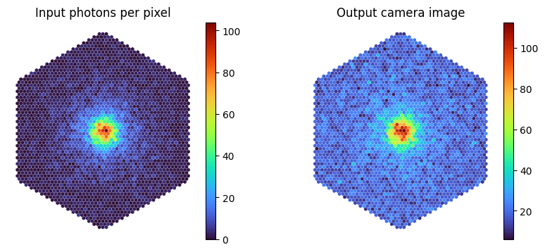
Compare input and output

We can now use camerashow to compare the number of detected photons with the image registered by the camera (which clearly shows a baseline shift due to the NSB)

fig, (ax1,ax2) = plt.subplots(1,2,figsize=(10,4))
cmap = 'turbo'

_ = camerashow(np.diff(pes[1]), cam_geo, cmap=cmap,ax=ax1)
_ = ax1.set_title('Input photons per pixel')

_ = camerashow(telescope.camera.images[0], cam_geo, cmap=cmap, ax=ax2)
_ = ax2.set_title('Output camera image')

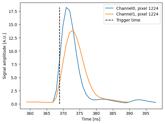
Inspect waveforms

Again, we can use the get_channel_signals() method to visualize the signal of a specific pixel (since the method returns a CuPy array, remember to use the get() method):

# Get the signal of each channel, shape (N-pixels, window size)
channel0 = camera.get_channel_signals(0,reshape=True)
channel1 = camera.get_channel_signals(1,reshape=True)

# Plot a pixel
pixel = 1224
pix_0 = channel0[pixel].get()
pix_1 = channel1[pixel].get()
plt.plot(camera.time_windows[0], pix_0, label=f'Channel0, pixel {pixel}')
plt.plot(camera.time_windows[1], pix_1, label=f'Channel1, pixel {pixel}')
plt.vlines(camera.trigger_time, 0, max(pix_0.max(), pix_1.max()), color='black', ls='--', label='Trigger time')

_ = plt.legend()
plt.xlabel('Time [ns]')
plt.ylabel('Signal amplitude [A.U.]')

Text(0, 0.5, 'Signal amplitude [A.U.]')

Simulate camera response directly using trace_photons()

trace_photons() can automatically handle the camera simulation when passing simulate_camera=True. In the following example we simulate the detection of multiple Guassian beams without manually calling camera.simulate_response(). Since the telscope is pointing at the horizon, the beams are generated randomly in the field of view:

telescope.camera.restart() # clear all images

# Clear benchmark measurements
telescope.timer.clear()
telescope.timer.active = True
telescope.camera.timer.clear()
telescope.camera.timer.active = True

for _ in range(100):
    n = np.random.poisson(200000)
    source.directions.altitude = telescope.altitude + np.random.normal(0, 2.5)
    source.directions.azimuth = telescope.azimuth + np.random.normal(0, 2.5)
    telescope.trace_photons(
        *source.generate(n),
        simulate_camera=True
    )

Inspect performance

In the previous cell we activated the timer attribute of camera and telescope. It is an istance of the BenchmarkTimer class, an utility class that allows the measurement of the elapsed time of different parts of the simulation.

Telescope report

telescope.timer.print_results()

Section	Measure	N calls	Mean (ms)	Median (ms)	Stdev (ms)	Min (ms)	Max (ms)
simulate_response	copy to device	100	0.065	0.039	0.078	0.036	0.400
simulate_response	weight photons	100	0.012	0.012	0.002	0.010	0.021
simulate_response	atmospheric transmission	100	0.013	0.013	0.002	0.011	0.022
simulate_response	trace onto focal plane	100	2.059	2.121	0.682	0.726	3.286
simulate_response	generate camera input	100	0.851	0.789	0.348	0.124	2.168
simulate_response	filter events to be simulated	100	0.136	0.110	0.119	0.021	1.021
simulate_response	simulate camera response	100	0.603	0.527	0.608	0.027	6.070
simulate_response	total_time	100	3.740	3.874	1.267	0.964	8.942

Camera report

telescope.camera.timer.print_results()

Section	Measure	N calls	Mean (ms)	Median (ms)	Stdev (ms)	Min (ms)	Max (ms)
simulate_response	get source	93	0.004	0.003	0.001	0.003	0.011
simulate_response	compute trigger windows	93	0.038	0.026	0.054	0.022	0.404
simulate_response	pre_trigger_action	93	0.157	0.142	0.054	0.127	0.575
simulate_response	trigger_action	93	0.223	0.141	0.585	0.132	5.820
simulate_response	post_trigger_action	93	0.001	0.001	0.000	0.001	0.003
simulate_response	compute sampling windows	70	0.006	0.005	0.001	0.005	0.010
simulate_response	pre_sampling_action	70	0.149	0.137	0.052	0.121	0.553
simulate_response	sampling_action	70	0.055	0.038	0.055	0.034	0.362
simulate_response	post_sampling_action	70	0.001	0.001	0.000	0.001	0.002
simulate_response	total_time	93	0.582	0.499	0.616	0.291	6.222
compute_signals[0]	windows_parameters	93	0.021	0.014	0.047	0.010	0.444
compute_signals[0]	signals allocation	93	0.003	0.003	0.001	0.002	0.006
compute_signals[0]	signals_parameters	93	0.001	0.001	0.000	0.001	0.002
compute_signals[0]	sipm_parameters	93	0.001	0.001	0.000	0.001	0.003
compute_signals[0]	background_parameters	93	0.005	0.005	0.001	0.005	0.010
compute_signals[0]	prepare_parameters	93	0.016	0.014	0.007	0.013	0.074
compute_signals[0]	compute_signals	93	0.108	0.101	0.023	0.090	0.284
compute_signals[0]	total_time	93	0.155	0.140	0.054	0.124	0.572
compute_signals[1]	windows_parameters	70	0.022	0.015	0.050	0.012	0.430
compute_signals[1]	signals allocation	70	0.003	0.003	0.000	0.002	0.004
compute_signals[1]	signals_parameters	70	0.001	0.001	0.000	0.001	0.001
compute_signals[1]	sipm_parameters	70	0.001	0.001	0.000	0.001	0.002
compute_signals[1]	background_parameters	70	0.005	0.005	0.001	0.004	0.008
compute_signals[1]	prepare_parameters	70	0.010	0.009	0.003	0.009	0.038
compute_signals[1]	compute_signals	70	0.104	0.100	0.012	0.087	0.147
compute_signals[1]	total_time	70	0.146	0.135	0.052	0.118	0.550

Visualize images

Another useful iactsim function is browse_images. This function allows to navigate through a set of images. For example the Guassian-beam images detected by the camera:

from iactsim.visualization import browse_images

browse_images(telescope.camera.images, cam_geo)

Pixel efficiency

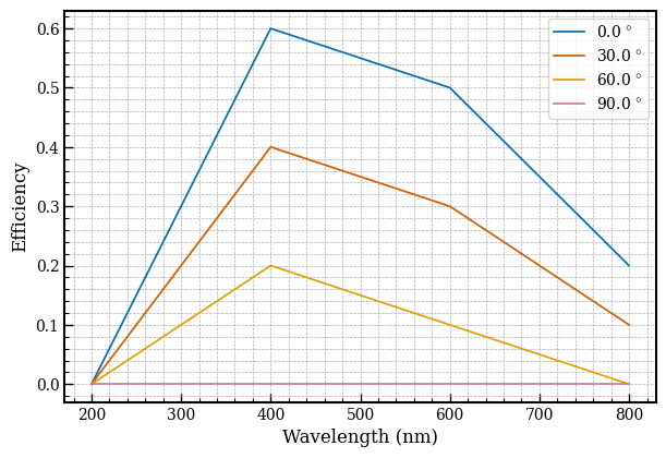
Each pixel can have its own efficiency as a function of wavelength and incidence angle. You can set the afficiency using the SurfaceProperties class:

from iactsim.optics import SurfaceProperties

pixel_prop = SurfaceProperties()
pixel_prop.efficiency_wavelength = [200,400,600,800]
pixel_prop.efficiency_incidence_angle = [0,30,60,90]
pixel_prop.efficiency = [
    [0., 0.6, 0.5, 0.2],
    [0., 0.4, 0.3, 0.1],
    [0., 0.2, 0.1, 0.0],
    [0., 0.0, 0.0, 0.0],
]

_ = pixel_prop.plot('eff')

Then assign the efficiency to the desired pixel (or you can use the same object on multiple pixels):

# Change the efficiency of the central pixel
pixels[1224].properties = pixel_prop

# This will pass the look-up table pointer to the ray-tracing kernel
telescope.cuda_init()

source.directions.altitude = telescope.altitude
source.directions.azimuth = telescope.azimuth
pes = telescope.trace_photons(
    *source.generate(300_000),
    get_camera_input=True
)
_ = camerashow(np.diff(pes[1]), cam_geo)

Pixel reflectance

If you want to take into account also pixel reflectance, you must declare the module as a REFLECTIVE_SENSITIVE surface, and define absorption and reflectance. For this kind of surface the transmittance is not used during the ray-tracing, while the absorption is computed as: \(a(\lambda,\theta)=1 - r(\lambda,\theta)\). The photon-detection efficiency is relative to the absorbed photons. So in this example the final efficiency, on-axis at 400 nm, is 0.8*0.6=0.48.

telescope.optical_system['Module0'].type = SurfaceType.REFLECTIVE_SENSITIVE

pixel_prop.wavelength = [300,900]
pixel_prop.absorption = [0.8,0.8]
pixel_prop.reflectance = [0.2,0.2]
pixels[1225].properties = pixel_prop

telescope.cuda_init()

pes = telescope.trace_photons(
    *source.generate(300_000),
    get_camera_input=True
)
_ = camerashow(np.diff(pes[1]), cam_geo)