Overview
iactsim is a high-performance Python package designed for simulating the response of Imaging Atmospheric Cherenkov Telescopes (IACTs). By exploiting the parallel computational power of GPUs (via CUDA and CuPy), it accelerates computationally intensive tasks such as ray-tracing and SiPM response simulation.
Package Structure
The framework is organized into four main modules:
optics: handles optical system, non-sequential ray-tracing and photon sources.
electronics: manages pixel signal generation, trigger logic and sampling logic. Currently only SiPM signal generation is supported, including prompt cross-talk, after-pulse and micro-cell recovery time.
visualization: provides tools for 3D geometry/ray-tracing rendering (via VTK) and helper matplotlib functions for data plotting.
iactxx: a general-purpose C++ extension module, currently used for high-performance parallel reading, decompression and conversion of files written with the IACT extension of CORSIKA7.
Key features
GPU Acceleration: accelerated performance for ray-tracing and camera response simulation using CUDA and CuPy.
Flexible Optics:
non-sequential ray-tracing algorithm supporting multiple reflections (e.g., protective windows, multi-layer coatings, SiPM reflectance);
currently supports spherical, aspherical, flat, cylindrical, cuboidal and conical surfaces;
flexible geometry modeling: supports surface segmentation where each segment is an independent surface, allowing for unique profiles (e.g., curvature variations) and customizable alignment errors (tilts/shifts);
Advanced Electronics:
detailed SiPM response simulation (prompt cross-talk, after-pulse and microcell recovery time);
run-time configuration of pixel properties on a per-pixel basis;
trigger and sampling logic customization.
Visualization:
built-in plotting capabilities for the detailed analysis of ray-tracing results and camera electronic signals;
3D interactive visualization of optical systems and photon paths using VTK.
Python-based: seamless integration with the scientific Python stack (NumPy, SciPy, Numba, Matplotlib, Jupyter, etc.).
Usage examples
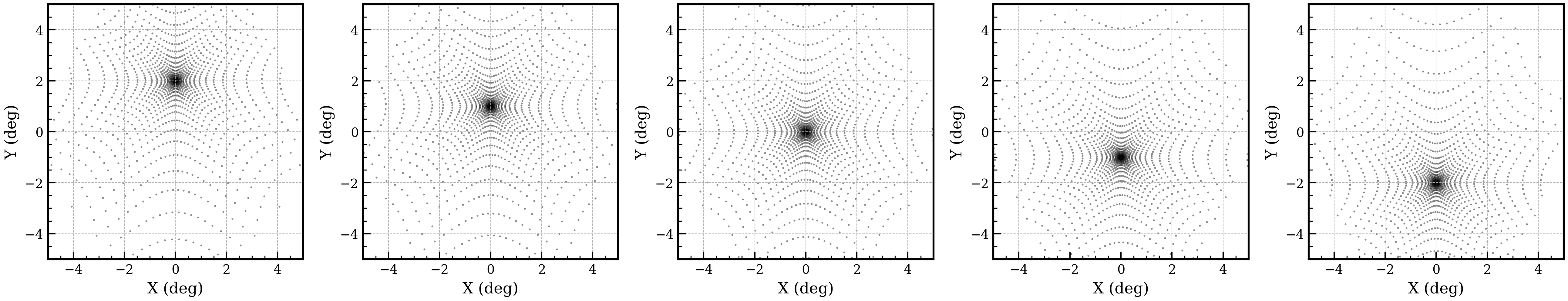
Optical system definition
import matplotlib.pyplot as plt
import iactsim
from iactsim.optics import (
    ApertureShape,
    SurfaceType,
    OpticalSystem,
)

# Use iactsim matplotlib style
plt.style.use('iactsim.iactsim')

# Spherical mirror
mirror_curvature_radius = 20000
plate_scale = mirror_curvature_radius/57.296/2.
mirror = iactsim.optics.SphericalSurface(
    half_aperture=10000.,
    curvature=1./mirror_curvature_radius,
    position=(0,0,0),
    # reflective in the pointing direction
    surface_type=SurfaceType.REFLECTIVE_FRONT,
    name = 'Mirror'
)

# Flat focal surface (5deg hexagon)
focal_plane = iactsim.optics.FlatSurface(
    half_aperture = 5*plate_scale,
    position = (0,0,0.5*mirror_curvature_radius),
    aperture_shape = ApertureShape.HEXAGONAL,
    # sensitive surface opposite to the pointing direction
    surface_type=SurfaceType.SENSITIVE_BACK,
    name = 'Focal Plane'
)

# Optical system
os = OpticalSystem(
    surfaces=[focal_plane, mirror],
    name='TEST-OS'
)

# Telescope position
pos = (0,0,0)

# Telescope pointing (alt,az)
poi = (0.,0.)

# IACT
telescope = iactsim.IACT(
    os,
    position=pos,
    pointing=poi
)

# Copy optical system data to the device
telescope.cuda_init()

# Photon source initialized on-axis
source = iactsim.optics.sources.Source(telescope)
source.positions.random = False # To make spot diagrams

# Plot spot diagram at different off-axis angles
n_plots = 5
fig, axes = plt.subplots(1,n_plots,figsize=(3.5*n_plots,3.5))

source.directions.altitude = telescope.altitude - 2.
for ax in axes:
    # Adjust photon position to match the mirror position
    source.set_target('Mirror')

    # Generate photons
    ps, vs, wls, ts = source.generate(10000)

    # Perform ray-tracing
    telescope.trace_photons(ps, vs, wls, ts)

    # Plot spot diagram
    iactsim.visualization.scatter(ps, s=0.2, ax=ax, color='black', alpha=0.5, scale=plate_scale)
    ax.set_xlabel('X (deg)')
    ax.set_ylabel('Y (deg)')
    ax.grid(ls='--')

    # Move the source
    source.directions.altitude += 1. # degree

plt.tight_layout()
plt.show()
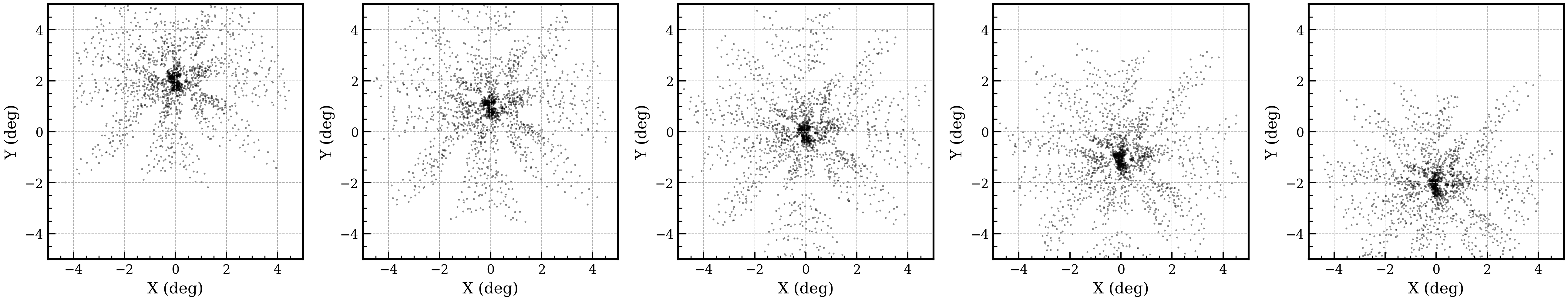
Mirror segmentation
The following code provides an example of how to segment a surface (AsphericalSurface, SphericalSurface or FlatSurface) starting from a mother surface (in this case mirror).
Note that each segment is an independent surface and does not need a mother surface, which is used here simply for convenience.
import numpy as np

# List of segments
segments = []

# Segment ID
k = 0

# Segments on a 10X10 grid, 80 total
n = 10
segment_distance = 2*mirror.half_aperture / (n+3)

for i in range(n+3):
    for j in range(n+3):
    offset = [
        -mirror.half_aperture+segment_distance*i,
        -mirror.half_aperture+segment_distance*j
    ]
    r_segment = np.sqrt(offset[0]**2+offset[1]**2)

    # Do not create segments outside the original mirror aperture
    if r_segment > mirror.half_aperture-segment_distance*np.sqrt(2):
        continue

    # Ideal segment position
    segment_position = [
        offset[0],
        offset[1],
        mirror.sagitta(r_segment),
    ]

    # Create the surface
    segment = iactsim.optics.SphericalSurface(
        curvature=mirror.curvature,
        half_aperture=0.45*segment_distance,
        position=segment_position,
        surface_type=mirror.type,
        name = f'Segment-{k}',
        aperture_shape=ApertureShape.SQUARE,
        # Big random dispersion for visualization purpose
        tilt_angles=np.random.normal(0,1,3),
        # Gaussian scattering
        scattering_dispersion=0.02
    )

    # Specify the segment offset
    # When a segment is created in this way:
    #  - it will be oriented with the same surface normal
    #    of the mother surface at the specified offset
    #  - `tilt_angles` attribute will define a deviation from this orientation.
    segment.offset = offset

    segments.append(segment)
    k += 1

# Optical system
segmented_os = iactsim.optics.OpticalSystem(
    surfaces=[focal_plane, *segments],
    name='SEGMENTED-TEST-OS'
)

# IACT
segmented_telescope = iactsim.IACT(segmented_os, position=pos, pointing=poi)
segmented_telescope.cuda_init()

# Plot spot diagram at different off-axis angles
n_plots = 5
fig, axes = plt.subplots(1,n_plots,figsize=(3.5*n_plots,3.5))

# Photon source initialized on-axis
source = iactsim.optics.sources.Source(segmented_telescope)
source.positions.radial_uniformity = False
source.positions.random = False
source.positions.r_max = mirror.half_aperture*1.5

source.directions.altitude -= 2.
for ax in axes:
    # Adjust photon position to match the mirror position
    source.set_target()

    # Generate photons
    ps, vs, wls, ts = source.generate(10000)

    # Perform ray-tracing
    segmented_telescope.trace_photons(ps, vs, wls, ts)

    # Plot spot diagram
    iactsim.visualization.scatter(ps, s=0.2, ax=ax, color='black', alpha=0.5, scale=plate_scale)
    ax.set_xlabel('X (deg)')
    ax.set_ylabel('Y (deg)')
    ax.grid(ls='--')

    # Move the source
    source.directions.altitude += 1. # degree

plt.tight_layout()
plt.show()
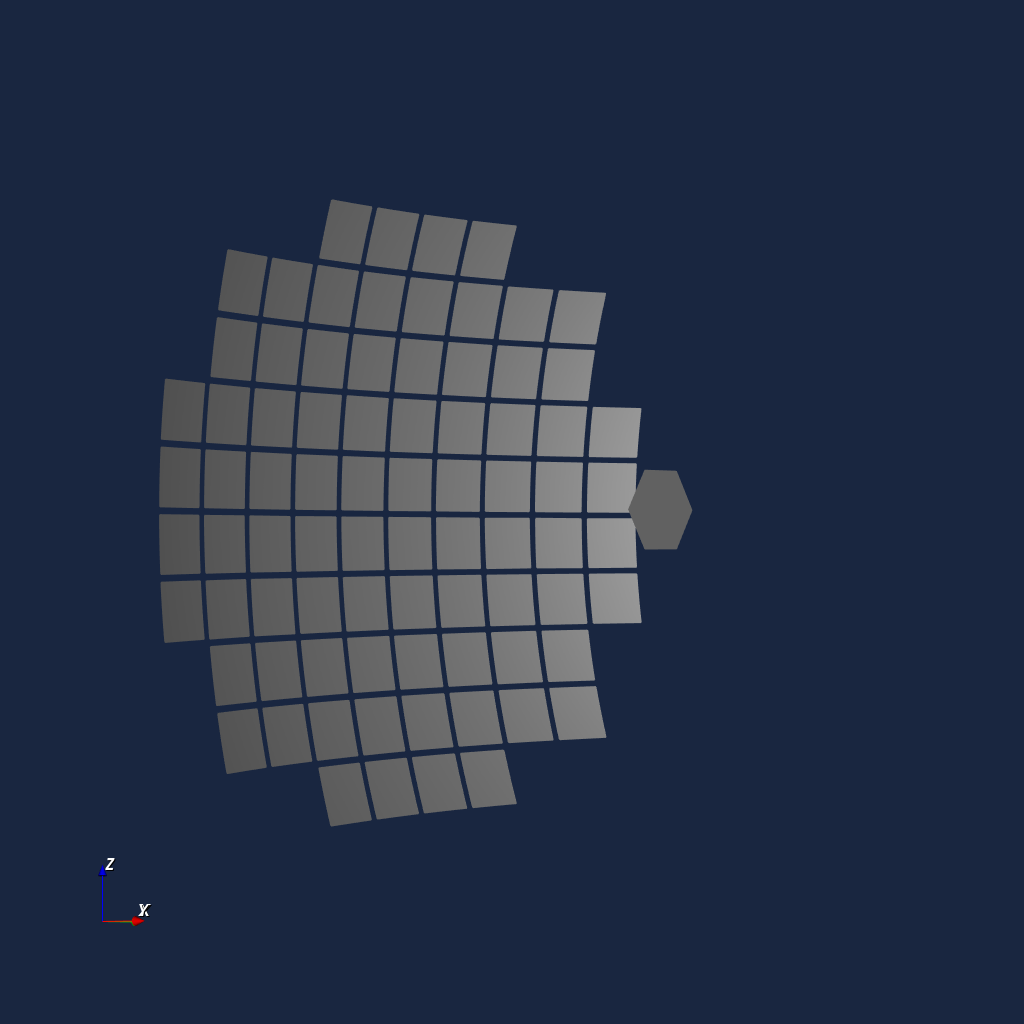
3D Visualization
Verify your geometry or visualize ray-tracing paths using the built-in VTK backend.
Interactive 3D view of the optical system
from iactsim.visualization import VTKOpticalSystem
renderer = VTKOpticalSystem(segmented_telescope.optical_system)
renderer.start_render()
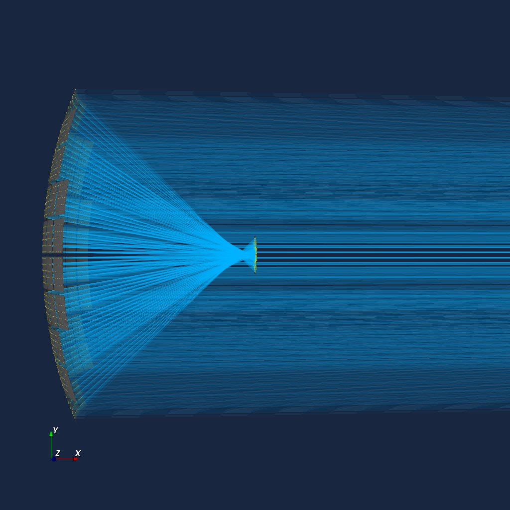
Visualize ray paths
segmented_telescope.visualize_ray_tracing(
    *source.generate(10000),
    map_wavelength_color=False,
    focal_point='Focal Plane',
    show_not_detected=False
)